devtools::install_github("LukeCe/spflow")Using github PAT from envvar GITHUB_PATSkipping install of 'spflow' from a github remote, the SHA1 (df913677) has not changed since last install.
Use `force = TRUE` to force installationSpatial Interaction Models have often used to explain origin-destination (OD) flows that arise in fields such as public bus commuting. These models rely on a function of the distance between the origin and destination as well as explanatory variables pertaining to characteristics of both origin and destination locations. Spatial interaction models assume that using distance as an explanatory variable will eradicate the spatial dependence among the sample of OD flows between pairs of locations. The notion that use of distance functions in conventional spatial interaction models effectively captures spatial dependence in interregional flows has long been challenged. In view of the limitation Spatial Interaction Models to account for spatial dependence, Spatial Econometric Interaction Models have been introduce James P. LeSage and R. Kelley Pace (2009).
In this in-class exercise, you will gain hands-on exercise on using spflow package, a R library specially developed for calibrating Spatial Econometric Interaction Models. By the end of this in-class exercise, you will acquire the skills to:
extract explanatory variables from secondary source,
assemble and derive explanatory variables from publicly available geospatial data,
integrate these explanatory variable into a tidy variables tibble data.frame.
calibrate Spatial Econometric Interaction Models by using spflow.
In this exercise, the development version (0.1.0.9010) of spflow will be used instead of the released version (0.1.0). The code chunk below will be used to install the development version of spflow package.
Using github PAT from envvar GITHUB_PATSkipping install of 'spflow' from a github remote, the SHA1 (df913677) has not changed since last install.
Use `force = TRUE` to force installationNext, will will load spflow and other R packages into R environment.
Before we can calibrate Spatial Econometric Interaction Models by using spflow package, three data sets are required. They are:
a spatial weights,
a tibble data.frame consists of the origins, destination, flows and distances between the origins and destination, and
a tibble data.frame consists of the explanatory variables.
For the purpose of this study, URA Master Planning 2019 Planning Subzone GIS data will be used.
In the code chunk below, MPSZ-2019 shapefile will be import into R environment as a sf tibble data.frame called mpsz.
mpsz <- st_read(dsn = "Take-home Exercise 2/data/geospatial",
                layer = "MPSZ-2019") %>%
  st_transform(crs = 3414)
Reading layer `MPSZ-2019' from data source
`D:\y1zaoWang\ISSS624\Take-home Exercise 2\data\geospatial'
using driver `ESRI Shapefile'
Simple feature collection with 332 features and 6 fields
Geometry type: MULTIPOLYGON
Dimension: XY
Bounding box: xmin: 103.6057 ymin: 1.158699 xmax: 104.0885 ymax: 1.470775
Geodetic CRS: WGS 84Next, the code chunk below will be used to import BusStop shapefile into R environment as an sf object called busstop.
busstop <- st_read(dsn = "Take-home Exercise 2/data/geospatial",
                   layer = "BusStop") %>%
  st_transform(crs = 3414)
Reading layer `BusStop' from data source
`D:\y1zaoWang\ISSS624\Take-home Exercise 2\data\geospatial'
using driver `ESRI Shapefile'
Simple feature collection with 5161 features and 3 fields
Geometry type: POINT
Dimension: XY
Bounding box: xmin: 3970.122 ymin: 26482.1 xmax: 48284.56 ymax: 52983.82
Projected CRS: SVY21In this study, our analysis will be focused on planning subzone with bus stop. In view of this, the code chunk below will be used to perform Point-in-Polygon count analysis.
Next, code chunk below will be used to select planning subzone with bus stops.
Simple feature collection with 314 features and 7 fields
Geometry type: MULTIPOLYGON
Dimension:     XY
Bounding box:  xmin: 2667.538 ymin: 21448.47 xmax: 55941.94 ymax: 50256.33
Projected CRS: SVY21 / Singapore TM
First 10 features:
            SUBZONE_N SUBZONE_C       PLN_AREA_N PLN_AREA_C       REGION_N
1    INSTITUTION HILL    RVSZ05     RIVER VALLEY         RV CENTRAL REGION
2      ROBERTSON QUAY    SRSZ01  SINGAPORE RIVER         SR CENTRAL REGION
3        FORT CANNING    MUSZ02           MUSEUM         MU CENTRAL REGION
4    MARINA EAST (MP)    MPSZ05    MARINE PARADE         MP CENTRAL REGION
5             SENTOSA    SISZ01 SOUTHERN ISLANDS         SI CENTRAL REGION
6      CITY TERMINALS    BMSZ17      BUKIT MERAH         BM CENTRAL REGION
7               ANSON    DTSZ10    DOWNTOWN CORE         DT CENTRAL REGION
8        STRAITS VIEW    SVSZ01     STRAITS VIEW         SV CENTRAL REGION
9     MARITIME SQUARE    BMSZ01      BUKIT MERAH         BM CENTRAL REGION
10 TELOK BLANGAH RISE    BMSZ15      BUKIT MERAH         BM CENTRAL REGION
   REGION_C                       geometry BUSSTOP_COUNT
1        CR MULTIPOLYGON (((28481.45 30...             2
2        CR MULTIPOLYGON (((28087.34 30...            10
3        CR MULTIPOLYGON (((29542.53 31...             6
4        CR MULTIPOLYGON (((35279.55 30...             2
5        CR MULTIPOLYGON (((26879.04 26...             1
6        CR MULTIPOLYGON (((27891.15 28...            10
7        CR MULTIPOLYGON (((29201.07 28...             5
8        CR MULTIPOLYGON (((31269.21 28...             4
9        CR MULTIPOLYGON (((26920.02 26...            21
10       CR MULTIPOLYGON (((27483.57 28...            11
Notice that there are 313 planning subzone in this sf object.
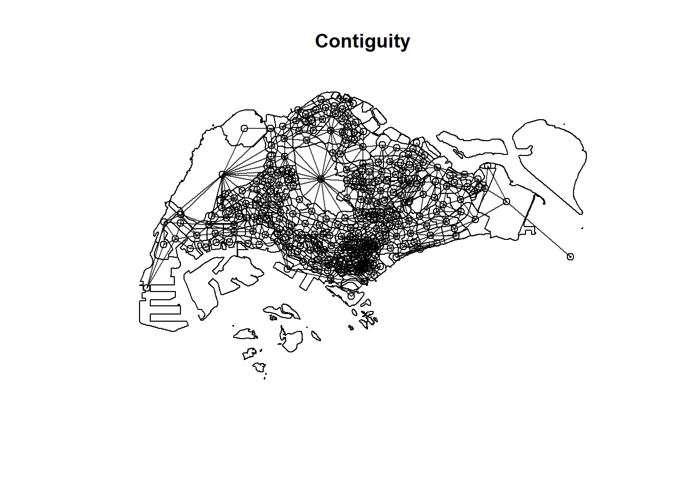
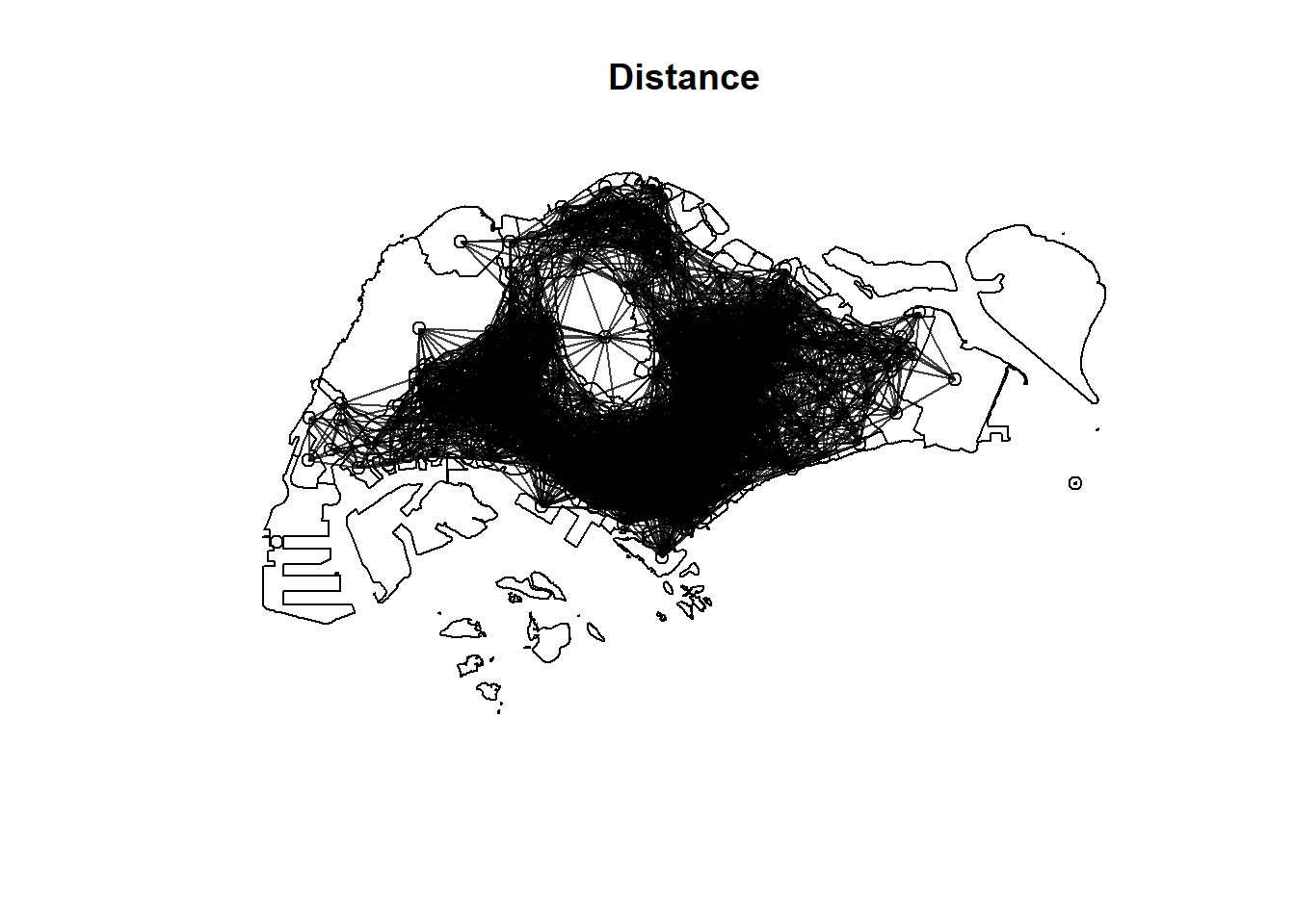
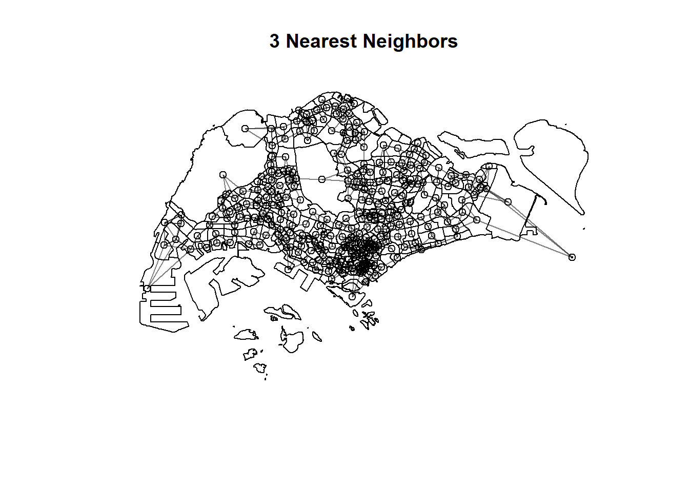
There are three different matrices that can be used to describe the connectivity between planning subzone. They are: contiguity, fixed distance and adaptive distance.
Code chunk below will be used to compute the three spatial weights at one goal.
$by_contiguity
Neighbour list object:
Number of regions: 314
Number of nonzero links: 1904
Percentage nonzero weights: 1.931113
Average number of links: 6.063694

$by_distance
Neighbour list object:
Number of regions: 314
Number of nonzero links: 15422
Percentage nonzero weights: 15.64161
Average number of links: 49.11465
2 regions with no links:
152 314
3 disjoint connected subgraphs

$by_knn
Neighbour list object:
Number of regions: 314
Number of nonzero links: 942
Percentage nonzero weights: 0.955414
Average number of links: 3
Non-symmetric neighbours list
Code chunks below will be used to plot the spatial weights in mpsz_nb.
plot(st_geometry(mpsz))
plot(mpsz_nb$by_contiguity,
     centroids,
     add = T,
     col = rgb(0,0,0,
               alpha=0.5))
title("Contiguity") 
plot(st_geometry(mpsz))
plot(mpsz_nb$by_distance,
     centroids,
     add = T,
     col = rgb(0,0,0,
               alpha=0.5))
title("Distance") 
plot(st_geometry(mpsz))
plot(mpsz_nb$by_knn,
     centroids,
     add = T,
     col = rgb(0,0,0,
               alpha=0.5))
title("3 Nearest Neighbors") 
When you are happy with the results, it is time to save mpsz_nb into an rds file for subsequent use by using the code chunk below.
In this section, you will learn how to prepare a flow data at the planning subzone level as shown in the screenshot below.
busstop_mpsz <- st_intersection(busstop, mpsz) %>%
  select(BUS_STOP_N, SUBZONE_C) %>%
  st_drop_geometry()
Warning: attribute variables are assumed to be spatially constant throughout
all geometriesNext, we are going to append the planning subzone code from busstop_mpsz data.frame onto odbus6_9 data frame.
od_data <- left_join(odbus6_9 , busstop_mpsz,
            by = c("ORIGIN_PT_CODE" = "BUS_STOP_N")) %>%
  rename(ORIGIN_BS = ORIGIN_PT_CODE,
         ORIGIN_SZ = SUBZONE_C,
         DESTIN_BS = DESTINATION_PT_CODE)
Warning in left_join(odbus6_9, busstop_mpsz, by = c(ORIGIN_PT_CODE = "BUS_STOP_N")): Detected an unexpected many-to-many relationship between `x` and `y`.
ℹ Row 25632 of `x` matches multiple rows in `y`.
ℹ Row 673 of `y` matches multiple rows in `x`.
ℹ If a many-to-many relationship is expected, set `relationship =
"many-to-many"` to silence this warning.Before continue, it is a good practice for us to check for duplicating records.
If duplicated records are found, the code chunk below will be used to retain the unique records.
It will be a good practice to confirm if the duplicating records issue has been addressed fully.
Next, we will update od_data data frame with the planning subzone codes.
Warning in left_join(od_data, busstop_mpsz, by = c(DESTIN_BS = "BUS_STOP_N")): Detected an unexpected many-to-many relationship between `x` and `y`.
ℹ Row 167 of `x` matches multiple rows in `y`.
ℹ Row 672 of `y` matches multiple rows in `x`.
ℹ If a many-to-many relationship is expected, set `relationship =
"many-to-many"` to silence this warning.od_data <- od_data %>%
rename(DESTIN_SZ = SUBZONE_C) %>%
drop_na() %>%
group_by(ORIGIN_SZ, DESTIN_SZ) %>%
summarise(TRIPS = sum(TRIPS))`summarise()` has grouped output by 'ORIGIN_SZ'. You can override using the
`.groups` argument.The od_data data.frame should look similar the table below.
| ORIGIN_SZ | DESTIN_SZ | TRIPS |
|---|---|---|
| AMSZ01 | AMSZ01 | 2694 |
| AMSZ01 | AMSZ02 | 10591 |
| AMSZ01 | AMSZ03 | 14980 |
| AMSZ01 | AMSZ04 | 3106 |
| AMSZ01 | AMSZ05 | 7734 |
In spatial interaction, a distance matrix is a table that shows the distance between pairs of locations. For example, in the table below we can see an Euclidean distance of 3926.0025 between MESZ01 and RVSZ05, of 3939.1079 between MESZ01 and SRSZ01, and so on. By definition, an location’s distance from itself, which is shown in the main diagonal of the table, is 0.
There are at least two ways to compute the required distance matrix. One is based on sf and the other is based on sp. Past experience shown that computing distance matrix by using sf function took relatively longer time that sp method especially the data set is large. In view of this, sp method is used in the code chunks below.
First as.Spatial() will be used to convert mpsz from sf tibble data frame to SpatialPolygonsDataFrame of sp object as shown in the code chunk below.
class       : SpatialPolygonsDataFrame
features    : 314
extent      : 2667.538, 55941.94, 21448.47, 50256.33  (xmin, xmax, ymin, ymax)
crs         : +proj=tmerc +lat_0=1.36666666666667 +lon_0=103.833333333333 +k=1 +x_0=28001.642 +y_0=38744.572 +ellps=WGS84 +towgs84=0,0,0,0,0,0,0 +units=m +no_defs
variables   : 7
names       : SUBZONE_N, SUBZONE_C, PLN_AREA_N, PLN_AREA_C,       REGION_N, REGION_C, BUSSTOP_COUNT
min values  : ADMIRALTY,    AMSZ01, ANG MO KIO,         AM, CENTRAL REGION,       CR,             1
max values : YUNNAN, YSSZ09, YISHUN, YS, WEST REGION, WR, 87 Next, spDists() of sp package will be used to compute the Euclidean distance between the centroids of the planning subzones.
           [,1]     [,2]      [,3]     [,4]     [,5]     [,6]     [,7]     [,8]
 [1,]    0.0000  305.737  951.8314 5254.066 4975.002 3176.159 2345.174 3455.579
 [2,]  305.7370    0.000 1045.9088 5299.849 4669.295 2873.497 2074.691 3277.921
 [3,]  951.8314 1045.909    0.0000 4303.232 5226.873 3341.212 2264.201 2890.870
 [4,] 5254.0664 5299.849 4303.2323    0.000 7707.091 6103.071 5007.197 3699.242
 [5,] 4975.0021 4669.295 5226.8731 7707.091    0.000 1893.049 3068.627 4009.437
 [6,] 3176.1592 2873.497 3341.2116 6103.071 1893.049    0.000 1200.264 2532.383
 [7,] 2345.1741 2074.691 2264.2014 5007.197 3068.627 1200.264    0.000 1709.443
 [8,] 3455.5791 3277.921 2890.8696 3699.242 4009.437 2532.383 1709.443    0.000
 [9,] 3860.6063 3612.345 4570.3316 8324.615 2766.650 2606.583 3383.338 5032.870
[10,] 2634.7332 2358.403 3255.0325 6981.431 2752.882 1666.022 2115.640 3815.333
          [,9]    [,10]
 [1,] 3860.606 2634.733
 [2,] 3612.345 2358.403
 [3,] 4570.332 3255.033
 [4,] 8324.615 6981.431
 [5,] 2766.650 2752.882
 [6,] 2606.583 1666.022
 [7,] 3383.338 2115.640
 [8,] 5032.870 3815.333
 [9,]    0.000 1357.426
[10,] 1357.426    0.000
Notice that the output dist is a matrix object class of R. Also notice that the column heanders and row headers are not labeled with the planning subzone codes.
First, we will create a list sorted according to the the distance matrix by planning sub-zone code.
Next we will attach SUBZONE_C to row and column for distance matrix matching ahead
Next, we will pivot the distance matrix into a long table by using the row and column subzone codes as show in the code chunk below.
     Var1   Var2  DISTANCE
1  RVSZ05 RVSZ05    0.0000
2  SRSZ01 RVSZ05  305.7370
3  MUSZ02 RVSZ05  951.8314
4  MPSZ05 RVSZ05 5254.0664
5  SISZ01 RVSZ05 4975.0021
6  BMSZ17 RVSZ05 3176.1592
7  DTSZ10 RVSZ05 2345.1741
8  SVSZ01 RVSZ05 3455.5791
9  BMSZ01 RVSZ05 3860.6063
10 BMSZ15 RVSZ05 2634.7332
The code chunk below is used to rename the origin and destination fields.
Now, left_join() of dplyr will be used to flow_data dataframe and distPair dataframe. The output is called flow_data1.
Joining with `by = join_by(ORIGIN_SZ, DESTIN_SZ)`The flow_data should look similar the table below.
| ORIGIN_SZ | DESTIN_SZ | DISTANCE | TRIPS |
|---|---|---|---|
| RVSZ05 | RVSZ05 | 0.0000 | 39 |
| SRSZ01 | RVSZ05 | 305.7370 | 1044 |
| MUSZ02 | RVSZ05 | 951.8314 | 83 |
| MPSZ05 | RVSZ05 | 5254.0664 | 0 |
| SISZ01 | RVSZ05 | 4975.0021 | 0 |
| BMSZ17 | RVSZ05 | 3176.1592 | 0 |
| DTSZ10 | RVSZ05 | 2345.1741 | 0 |
| SVSZ01 | RVSZ05 | 3455.5791 | 0 |
| BMSZ01 | RVSZ05 | 3860.6063 | 0 |
| BMSZ15 | RVSZ05 | 2634.7332 | 0 |
Before moving on to the next task, let’s save flow_data into an rds file by usign the code chunk below.
The third input data of spflow is a data.frame that contains all the explanatory variables of the geographical unit (i.e. Planning Subzone).
For the purpose of this exercise, we will include three population age-groups as the explanatory variables. They are population age 7-12, 13-24, and 25-64. These information are available in a data file called pop.csv.
The code chunk below will be used to import pop.csv into R environment and save it as an tibble data.frame object called pop.
Rows: 332 Columns: 5
── Column specification ────────────────────────────────────────────────────────
Delimiter: ","
chr (2): PA, SZ
dbl (3): AGE7_12, AGE13_24, AGE25_64

ℹ Use `spec()` to retrieve the full column specification for this data.
ℹ Specify the column types or set `show_col_types = FALSE` to quiet this message.| SZ_NAME | SZ_CODE | BUSSTOP_COUNT | AGE7_12 | AGE13_24 | AGE25_64 | geometry |
|---|---|---|---|---|---|---|
| INSTITUTION HILL | RVSZ05 | 2 | 330 | 360 | 2260 | MULTIPOLYGON (((28481.45 30… |
| ROBERTSON QUAY | SRSZ01 | 10 | 320 | 350 | 2200 | MULTIPOLYGON (((28087.34 30… |
| FORT CANNING | MUSZ02 | 6 | 0 | 10 | 30 | MULTIPOLYGON (((29542.53 31… |
| MARINA EAST (MP) | MPSZ05 | 2 | 0 | 0 | 0 | MULTIPOLYGON (((35279.55 30… |
| SENTOSA | SISZ01 | 1 | 200 | 260 | 1440 | MULTIPOLYGON (((26879.04 26… |
| CITY TERMINALS | BMSZ17 | 10 | 0 | 0 | 0 | MULTIPOLYGON (((27891.15 28… |
First, we will import schools.rds into R environment.
The, code chunk below will be used to perform Point-in-Polygon count analysis and save the derived values into a new field of mpsz_var called SCHOOL_COUNT.
Next, we will import the rest of the shapefiles into R environemnt using the code chunk below.
business <- st_read(dsn = "In-class_Ex5/data/geospatial",
                    layer = "Business") %>%
  st_transform(crs = 3414)
Reading layer `Business' from data source
`D:\y1zaoWang\ISSS624\In-class_Ex5\data\geospatial' using driver `ESRI Shapefile'
Simple feature collection with 6550 features and 3 fields
Geometry type: POINT
Dimension: XY
Bounding box: xmin: 3669.148 ymin: 25408.41 xmax: 47034.83 ymax: 50148.54
Projected CRS: SVY21 / Singapore TMretails <- st_read(dsn = "In-class_Ex5/data/geospatial",
layer = "Retails") %>%
st_transform(crs = 3414)Reading layer `Retails' from data source
`D:\y1zaoWang\ISSS624\In-class_Ex5\data\geospatial' using driver `ESRI Shapefile'
Simple feature collection with 37635 features and 3 fields
Geometry type: POINT
Dimension: XY
Bounding box: xmin: 4737.982 ymin: 25171.88 xmax: 48265.04 ymax: 50135.28
Projected CRS: SVY21 / Singapore TMfinserv <- st_read(dsn = "In-class_Ex5/data/geospatial",
layer = "FinServ") %>%
st_transform(crs = 3414)Reading layer `FinServ' from data source
`D:\y1zaoWang\ISSS624\In-class_Ex5\data\geospatial' using driver `ESRI Shapefile'
Simple feature collection with 3320 features and 3 fields
Geometry type: POINT
Dimension: XY
Bounding box: xmin: 4881.527 ymin: 25171.88 xmax: 46526.16 ymax: 49338.02
Projected CRS: SVY21 / Singapore TMentertn <- st_read(dsn = "In-class_Ex5/data/geospatial",
layer = "entertn") %>%
st_transform(crs = 3414)Reading layer `entertn' from data source
`D:\y1zaoWang\ISSS624\In-class_Ex5\data\geospatial' using driver `ESRI Shapefile'
Simple feature collection with 114 features and 3 fields
Geometry type: POINT
Dimension: XY
Bounding box: xmin: 10809.34 ymin: 26528.63 xmax: 41600.62 ymax: 46375.77
Projected CRS: SVY21 / Singapore TMReading layer `F&B' from data source
`D:\y1zaoWang\ISSS624\In-class_Ex5\data\geospatial' using driver `ESRI Shapefile'
Simple feature collection with 1919 features and 3 fields
Geometry type: POINT
Dimension: XY
Bounding box: xmin: 6010.495 ymin: 25343.27 xmax: 45462.43 ymax: 48796.21
Projected CRS: SVY21 / Singapore TMlr <- st_read(dsn = "In-class_Ex5/data/geospatial",
layer = "Liesure&Recreation") %>%
st_transform(crs = 3414)Reading layer `Liesure&Recreation' from data source
`D:\y1zaoWang\ISSS624\In-class_Ex5\data\geospatial' using driver `ESRI Shapefile'
Simple feature collection with 1217 features and 30 fields
Geometry type: POINT
Dimension: XY
Bounding box: xmin: 6010.495 ymin: 25134.28 xmax: 48439.77 ymax: 50078.88
Projected CRS: SVY21 / Singapore TMThen,we will perform Point-in-Polygon analysis for each of these sf object by using the code chunk below.
mpsz_var$`BUSINESS_COUNT`<- lengths(
  st_intersects(
    mpsz_var, business))

mpsz_var$`RETAILS_COUNT`<- lengths(
  st_intersects(
    mpsz_var, retails))

mpsz_var$`FINSERV_COUNT`<- lengths(
  st_intersects(
    mpsz_var, finserv))

mpsz_var$`ENTERTN_COUNT`<- lengths(
  st_intersects(
    mpsz_var, entertn))

mpsz_var$`FB_COUNT`<- lengths(
  st_intersects(
    mpsz_var, fb))

mpsz_var$`LR_COUNT`<- lengths(
  st_intersects(
mpsz_var, lr))Rows: 314
Columns: 14
$ SZ_NAME <chr> "INSTITUTION HILL", "ROBERTSON QUAY", "FORT CANNING", "…
$ SZ_CODE <chr> "RVSZ05", "SRSZ01", "MUSZ02", "MPSZ05", "SISZ01", "BMSZ…
$ BUSSTOP_COUNT <int> 2, 10, 6, 2, 1, 10, 5, 4, 21, 11, 2, 9, 6, 1, 4, 7, 24,…
$ AGE7_12 <dbl> 330, 320, 0, 0, 200, 0, 0, 0, 350, 470, 0, 300, 390, 0,…
$ AGE13_24 <dbl> 360, 350, 10, 0, 260, 0, 0, 0, 460, 1160, 0, 760, 890, …
$ AGE25_64 <dbl> 2260, 2200, 30, 0, 1440, 0, 0, 0, 2600, 6260, 630, 4350…
$ geometry <MULTIPOLYGON [m]> MULTIPOLYGON (((28481.45 30..., MULTIPOLYG…
$ SCHOOL_COUNT <int> 1, 0, 0, 0, 0, 0, 0, 0, 0, 2, 0, 1, 1, 0, 0, 0, 1, 0, 0…
$ BUSINESS_COUNT <int> 6, 4, 7, 0, 1, 11, 15, 1, 10, 1, 17, 6, 0, 0, 51, 2, 3,…
$ RETAILS_COUNT <int> 26, 207, 17, 0, 84, 14, 52, 0, 460, 34, 263, 55, 37, 1,…
$ FINSERV_COUNT <int> 3, 18, 0, 0, 29, 4, 6, 0, 34, 4, 26, 4, 3, 6, 59, 3, 8,…
$ ENTERTN_COUNT <int> 0, 6, 3, 0, 2, 0, 0, 0, 1, 0, 0, 0, 0, 0, 3, 0, 0, 0, 0…
$ FB_COUNT <int> 4, 38, 4, 0, 38, 15, 5, 0, 20, 0, 9, 25, 0, 0, 9, 1, 3,…
$ LR_COUNT <int> 3, 11, 7, 0, 20, 0, 0, 0, 19, 2, 4, 4, 1, 1, 13, 0, 17,…Three spflow objects are required, they are:
spflow_network-class, an S4 class that contains all information on a spatial network which is composed by a set of nodes that are linked by some neighborhood relation.
spflow_network_pair-class, an S4 class which holds information on origin-destination (OD) pairs. Each OD pair is composed of two nodes, each belonging to one network. All origin nodes must belong to the same origin network should be contained in one spflow_network-class, and likewise for the destinations.
spflow_network_multi-class, an S4 class that gathers information on multiple objects of types spflow_network-class and spflow_network_pair-class. Its purpose is to ensure that the identification between the nodes that serve as origins or destinations, and the OD-pairs is consistent (similar to relational data bases).
Let us retrieve by using the code chunk below